This is a guest article from Yoav Ezer. If you want to guest post on this blog, check out the guidelines here.

The IF() function is one of Excel’s super functions. It is a fundamental building-block of Excel formulas. You will find it present in almost any complex formula. There is a lot more power in Excel formulas conditions than just the basic IF() function, though.

Here are 7 conditional techniques that can help you create even more robust and useful Excel formulas:

1. Nested If Functions

This is the most basic type of ‘complex’ if() function. You can use an additional if function to create a more complex condition within your Excel formula.

For instance:

=IF(A1>10,IF(A1<20,"In range"))

The function above would test whether cell A1 contains a value that’s between 10 and 20. Only if both conditions are satisfied then the formula returns the value “In range”.

It is possible to use several levels of IF() function nesting. For example:

=IF(A1>10,IF(A1<20,IF(B2="HAS AMMO","FIRE!!!!")))

The formula above tests that A1 contains a number that is within range and that B2 holds the status ‘HAS AMMO’ and only if those three conditions are satisfied, it returns a value of “FIRE!”.

2. Logical-Boolean Functions

Nesting is powerful but it is complicated and often results in a formula that is difficult to read or change. A much better way to create complex conditions is to use Excel’s Boolean functions.

The AND() function will return true if all its parameters are true conditions.

So, the formula…

=IF(AND(A1>10,A1<20), "In range")

Will also check if cell A1 is between 10 and 20 pluse, it is much easier to understand (and to write) then the nested formula above.

The following formula…

=IF(AND(A1>10,A2<20,B1="HAS AMMO"),"FIRE!")

Is ten times easier to write/read then the corresponding nested IF() above

Another extremely useful Boolean function is the OR() function.

The formula…

=IF(OR(A1="CAT IS AWAY",A1="CAT IS BUSY"),"THE MICE PLAY")

Will return ‘THE MICE PLAY’ if A1 equals either ‘cat is away’ or ‘cat is busy’.

3. Countif, SumIf, Averageif, etc.

This group of functions allows you to apply a range function such as SUM(), COUNT() OR AVERAGE() only to rows that meet a specific condition.

For instance, you can sum or count all the sales that were made during the year 2001 as shown below:

It goes without saying that these conditional functions are very useful.

4. Countifs, SumIfs, Averageifs, etc.

The COUNTIFS() and SUMIFS() function (and the rest of the multiple conditions aggregate functions) were introduced in Excel 2007.

These functions enable us to apply an aggregation function to a subset of rows where those rows meet several conditions.

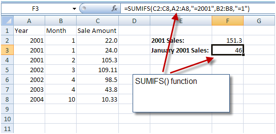
For instance, we can use the SUMIFS() function to sum all the sales that were made in the January of 2001, with a single function…

5. If and Array Formulas

Array formulas might be the most advanced of the formula techniques and while we can’t hope to cover the topic of array formulas in this article, it is important to mention that combining the IF() function with array formulas is a powerful tool.

In Excel versions prior to 2007, the formula AVERAGEIF() did not exist. So, if for example, you wished to average a range of numbers without including Zeros in the calculation, you needed to rely on an array formula:

Array formulas can also be used to mimic the working of countifs(), sumifs() and the rest of the xxxxxifs() functions, that simply did not exist in Excel versions before 2007.

They can also be used to implement new functions that does not exist such as MAXIF() and MINIF().

For a more in depth discussion of array formulas, look here.

6. IFError() function

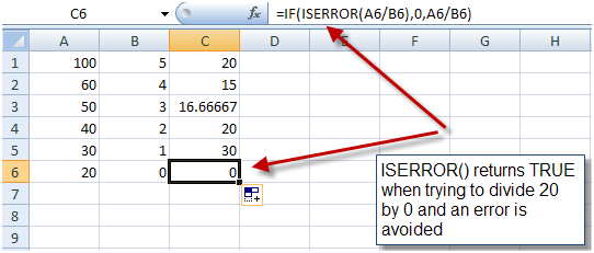
A close relative of the IF() function is the IFERROR() function. It allows you return a valid value in case a formula returns an error. For instance, if you have a formula that might cause a division by zero error, you can use the IFERROR() function to catch this event and return a valid value, as shown below:

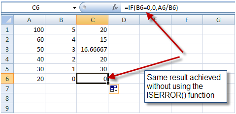
Note: It is better to use the IF() function to avoid an error then to use the ISERROR() function to catch an error. It is both faster (in terms of CPU) and better programming practice. So the same result we achieved with the ISERROR() function above can be achieved with an IF() function as shown here:

But there are cases when you cannot pretest the formula parameters and in those cases the ISERROR() function can come in handy.

7. Information functions

Distant relatives of the IF() function are the information functions. This group includes several functions that give you information about the type of the value contained in a cell (if it’s a string, a number, an odd number or an even number), if a cell is empty or if it contains an N/A value and more.

These functions, when used in conjunction with the IF() function can be pretty handy, for example, they allow you to easily check whether a cell is empty:

Summary

Our examples in this article only scratch the surface, we would encourage you to experiment more into what you can do. These seven simple functions hide a great deal of power and utility.

They are the building blocks of some very useful macros. We hope we have inspired you to put them to use in your own projects!

More Excel tips:

1. How to work with Date functions in Excel
2. Create an Interactive Timeline with Microsoft Excel

Yoav is the CEO of Cogniview, a company that creates PDF to XLS conversion software. Prior to that, Yoav Ezer was the CEO of Nocturnus, a technology-centered software solution company. For more Excel tips from Yoav, join him on Facebook or Twitter.